Our goal – Mission
An alteration induced in a stable system configuration may give rise to systemic competition between stocks, and consequent proliferation of one to the expenses of the others. This leads to the destruction of the remnants of the system. When this happens in human, we call it cancer. H.T. Odum
The Centre fo the Study of the Systemic Dynamics of Complex Diseases (SMAC) was born in 2022, after a group of scholars coming from various different scientific disciplines started working on an innovative idea, aimed at developing a novel approach in the biomedicine research, in particular, in the study of complex diseases. These are incurable and poorly understood diseases – such as for example self-immune ones and some forms of liquid cancer – whose evolution emerges as a systemic manifestation of a complex dynamics, ruled by multiple feedbacks and crossing over any description based on classical linear chains of cause-effect.
As a matter of fact, several incurable diseases exhibit peculiar behaviours that are are still under debate even in their very description. For example, the mechanisms of treatment failure and the origin of non-genetic plasticity of tumour cells have not been comprehensively addressed yet. If Systems Biology is expected to move towards Systems Medicine, we need to balance the pathway-centric approaches focusing on cellular and biochemical mechanisms with structural law-like principles coming from systemic descriptions. Systems Thinking (ST), used in the quantitative approach given by stock-flow formalism, is in this sense the good candidate to develop this program. In particular, it allows a dynamic description of a disease, opening the door to an analytical representation of its evolution scenarios also accounting for different systemic timescales.
The first basic conception is to treat the complex disease as an emerging systemic property, ruled by the network of feedbacks operated at different hierarchical levels, and describe it using the conceptual and analytical formalism already used for studying the dynamics of complex ecosystems. As is typical of complexity, the system itself represents the real cause of its own behaviour: the study of how a disease system self-organizes, evolves and accesses new dynamic configurations, triggered by genetic mutation, is thus the actual focus of the proposed approach. The studied system therefore is not the cancer cell, the genome, the tissues, the organs, the patient or a set of patients, but the disease itself, properly described by diagrams and equations that overlook the details of the biochemistry of what happens, in order to represent at a higher hierarchical level how the whole system works and evolves. The pattern of feedbacks connecting the elements of the system is the feature that ultimately defines the systems dynamics, responsible of any change of its state upon change of external or internal conditions. Thus, we are not interested in what are the actual biophysical and biochemical mechanisms of the feedback controls, but rather to set up a system of interconnected differential equations representing the patterns of functioning and, from this, the set of configurations which the system itself has access to. In fact, the evolution of a complex system is a systemic property, not the property of local occurring in the system. Complex diseases are therefore those ones whose setting and evolution rely on the systemic configuration structures, whose dynamics is determined by the complexity of the feedbacks network that rule the matter, energy and information flows between the system’s elements. Inn this sense, genome mutations are not to be considered – from a systemic point of view – “the cause of the disease”, since the presence of a single mutation is not sufficient – for example – to make multiple myeloma set up. Instead, genome has the systemic role of providing the system of the access to new possible configurations and patterns, that “are” the disease. Therefore, the genome should not be considered a systemic input, despite its ultimate responsibility for the disease manifestation.
A correct identification of the accessible dynamical patterns would then allow to understand how the system works, and possibly to find the proper leverage points for intervening. It is important to further clarify that the words “system” and “systemic” as used in the actual ST framework have not the same meaning they assume in a System Biology (SB) context, and in general within the related computational approaches. While both SB and ST aim at describing a system as a whole, the former still retains the scale of the microlevel, in as much it considers a system as the collection of a large number of elements, whose dynamics is investigated thanks to the availability of big data and sophisticated mathematical and statistical tools. On the contrary, ST approach starts from the identification of a limited number of state variables, those necessary to model the resource flows and the feedback networks that describe the configuration patterns of the system dynamics. Network analysis, agent-based modelling, causal loop diagrams, while effectively describing the complexity of a system, may not capture the complexity of its dynamics.
The proposed approach is at the same time profoundly abstract in nature and strongly connected to the experimental observation and activity. Nevertheless, more than clinical (big) data we aim at simulating the variety of dynamic behaviours of the disease, including the rearrangement following the action of external driving forces such as drugs. In this respect, evolutionary and ecological linguistic framework and features can be considered for a new and general taxonomy of cancer, able to capture its variety form a structural point of view. In fact, systemic ecologists use stock-flow ST in the study of ecosystems, whose complexity in managing the resources is more than a metaphor for complex diseases.
Generally speaking, ST shifts the attention from the study of events, in terms of causes, effects and mutual relationships, to the study of the systems from which they emerge, in terms of feedback configurations, patterns, structures and leverage points. Figure 1 shows the famous iceberg-like pictorial representation of ST conception.
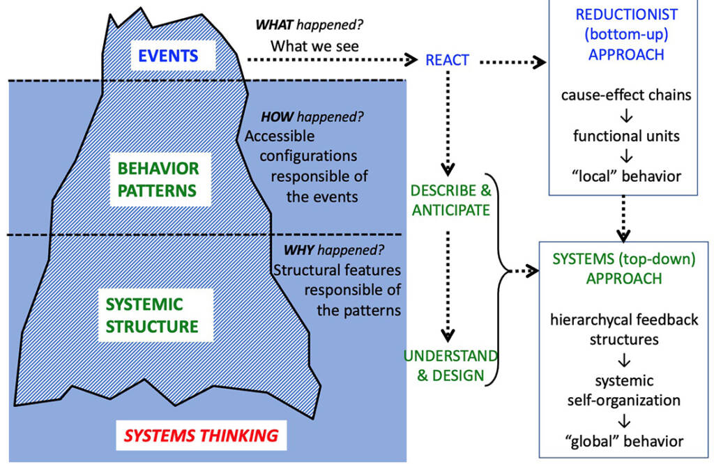
The basic idea is to replace (or at least to put together) the traditional bottom-up approach – that describes “local” behaviours through cause-effect chains and functional units – with a top-down approach that points out at the global behaviour of the system in terms of its operational configurations and accessible dynamic patterns, emerging from the feedback-driven self-organization. ST analysis can be connected to physical principles, among which the maximization of power (or em-power) is probably the most important: in the words by H.T. Odum, “In the competition among self-organizing processes, network designs that maximize empower will prevail, by reinforcing resource intake at the optimum efficiency”. Thermodynamics is therefore the natural conceptual framework for the development of a systemic approach different from those based on big data, so providing the ST – besides the epistemological – also a theoretical valence.
In the ST framework, a pivotal role is played by the creation of systemic diagrams, that play also the epistemic role of clarifying what are the feedbacks loops operating the system. putting the basis for the setting up of analytical and computational models. Generally speaking, ST shifts the attention from the study of local events, in terms of causes, effects and mutual relationships, to the study of the systemic patterns from which they emerge, in terms of feedback configurations, structures and leverage points. Contrary to Casual Loop Diagrams or other Networks-based diagrams, in the stock-flow representations a system is defined by a set of stocks (extensive variables) and the relative inflows and outflows, whose mutual controls set up the feedbacks network characteristic of the system at issue. Feedbacks may be direct (a stock influences a flow that influences the same stock) or indirect, when the mutual cause-effect relationship between the changes in flow and stock values follows a path that includes other stocks. This defines in turn a feedbacks hierarchy in the system, since their respective action manifest at different time scales. The pattern of feedbacks is therefore the feature that defines the systems dynamics, and it is responsible of any change in the system state upon the change of external or internal condition.
Inside a system, stocks are elements which contain a quantity of something (material, energy, information, money, entities, people…). A stock changes over time only through the action of flows (inflows and/or outflows), and may therefore act as delay or buffer or shock absorber for the system. The stocks content must be countable extensive state variables Qi, i=1,2,…,n, that constitute an n-tuple of numbers that at any time represents the state of the system. The choice of the set of variables depends on the hierarchical level of the desired description as well as on the overall purpose of the study. In fact, this choice reflects our need to describe the mechanisms by which the systems work and evolve. A stock may therefore represent a physically located set of something, but also a virtual set of elements that play a specific role in the system dynamics without having a corresponding specific location in the system (e.g., a stock of antibodies, of nutrients, etc.).
ST diagramming is flexible in terms of stocks definition, allowing to tailor the systemic representation depending on the object and the purpose of the study at issue. In this sense, for example, one could choose to diagram the system “blood” as a sub-system of “immune system”, but also vice-versa. Moreover, as said, stocks may have a physical location (e.g., stock of DNA inside a cell) or be distributed in the whole organism (e.g., stock of water). The set of stocks is then a numerical description of the system/disease state in its own states space, contrary to the NA descriptions made of edges that connect vertices, that aim at describing existing links to form a network for which big data are or may be available. It is worth stressing that, in our approach, the disease description will include stocks that apparently are not relevant from a clinical point of view, because they might be relevant in the onset of the systemic configurations typical of the disease. This way of describing a disease may result scarcely intuitive, but this is due to the mindset of considering what is actually a systemic property (a complex disease) as a linear cause-effect chain.
A stock may change its value only upon its inflows and/or outflows, represented by arrows entering or exiting the stock. Inflows and outflows are expressed as dQ/dt. In a stationary state of the system, stocks values are constant, or regularly oscillating. ST representation allows to describe analytically the role played by the various flows not only in terms of connected stocks, but also in terms of control or activation actions in the processes that affect different flows. In biological system, flows are of two types, those of matter (energy), that constitute the mechanism by which a stock value may change in time, and those of information (carried for example by proteins), responsible for the possible control action exerted by stocks on the processes that in turn control the flows. The specification of the control flows network is a fundamental aspect of systemic diagramming, since their action is responsible of feedbacks formation at different time scales.
Processes are any occurrence capable to alter – either quantitatively or qualitatively – a flow, by the action of one or more system stocks. Processes are then all what happens inside a system that either allows the stationarity of its state or let the system evolve toward a different configuration. Since the system state is a collection of stock values, and the only way to change the value of a stock is acting on its in/outflows, processes are located along the flows lines. Even the location of a process in the diagram does not have in general any correspondence in a physical location in real space. It is worth stressing that the processes entering the ST models are not just a – possibly exhaustive – collection of actual well-defined biological processes. What they must represent exhaustively is rather the network of interaction between the stocks that determines the dynamics and the configurations accessible to the system. A systemic process may be set to represent several different phenomena occurring at the same time, even possibly located in different physical places inside the real system whose diagram constitutes its representation. This is important since both the conceptual and the operational characters of the ST approach are based on this unconventional mindset.
As already said, the system boundary is not a physical one: as is typical of Systems Thinking, it is chosen to specify what are the main inflows that operate the systemic dynamics, and what are the system outputs. Figure 2 shows the main symbols we use in stock-flow diagrams. They are borrowed from the energy language, where shields indicate the stocks, circles the sources of something, line arrows the flows, solid arrows the processes, and the smooth grey rectangle the system boundary.
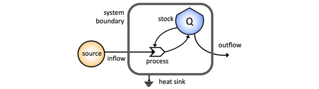
The figure depicts a simple system made by only one stock Q undergoing the action of a positive feedback, manifested by the mutual reinforcement of the stock Q and its inflow. For the second principle of thermodynamics, some energy is lost, and this is represented by the flow going down to the earth symbol (heat sink). The balancing between the relative strengths of the feedback and of the outflow will determine the evolution of the stock value.
Again, it must be stressed that the diagram representation is not a “photograph” of a set of elements that exist in this form and configuration in real space, but rather an abstract description aimed at taking a photograph of its dynamics. The analytical model of a system is derived directly from attributing a proper analytical form to the flows in the diagram, as well as to the type of interaction realized in each of the processes. From these, a charge-discharge equation will be set up for any of the n stocks defining the system state. The equation for the i-th stock change has the general form:
dQi/dt = (SaJain– SbJbout)i = f(Q1,…,Qn),
where inflows or the outflows are added for the stock at issue, and f is some specific functional dependence. In ST modelling, the equations are as a first approximation linearized, dQ/dt=kQ, with k=relative growth rate, constant. For small intervals of the variables during the time-step of the analyses, combined linear relations well represent the flows, even without using complex functions. This is typical for example of non-equilibrium thermodynamics, where flows depending on potential gradients are expressed using phenomenological constant coefficients. The quantity stored in a stock plays the role of a generalised force on the outflow in the same sense used in thermodynamic phenomenology, where non-equilibrium laws are set to correlate gradients of quantities (fluxes) to generalised forces via linear equations. The outflow from a single stock is therefore assumed to be proportional to the stock value. Indeed, most of the natural flows of energy or matter (anyhow accompanied by energy) are effectively covered by combinations of linear laws, thus validating the use of energy circuit symbolism to trace the flow paths connecting the stocks and the processes. In this conceptual framework, the flexibility of the circuit symbolism allows however to account for non-linear behaviours, for example, using switch symbols (operator) where a threshold step-wise dependence has to be accounted for. In fact, while the graphic model represents the circuit analogue description of the existing system, the equations are set to represent its actual dynamics. Indeed, a systemic model does not uniquely determine a network, but only an equivalence class of dynamically similar networks.
In figure 3, some simple “building blocks” are shown for situations that often occur in more complex real systems, namely, competition and cooperation situations involving two stocks, possibly representing stocks of different cells.
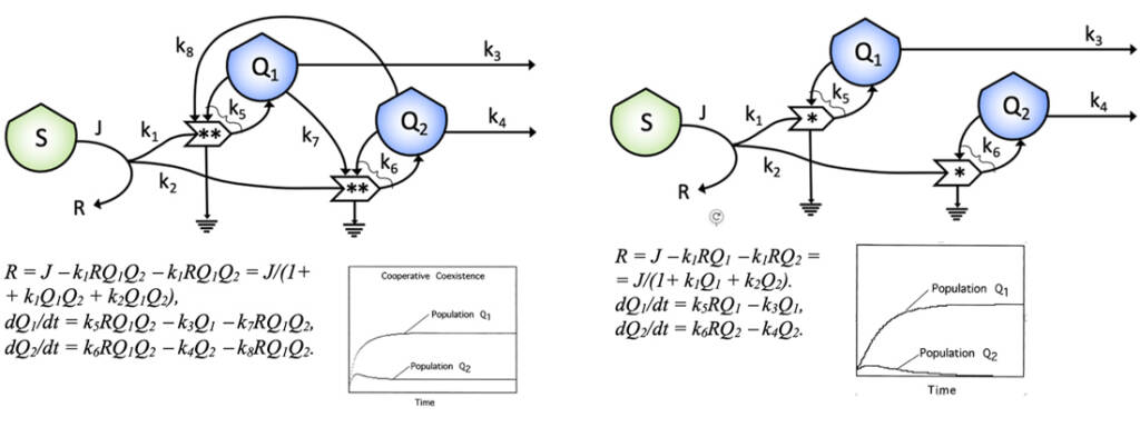
In this diagrams, stationary states (constant or regularly oscillating stock values) may be used to calibrate the equations under the constraints of energy and mass conservation. On the other hand, flows balancing description does not capture the mutual causality between the stocks values given by the loops, that represents the complexity of the feedback-driven dynamics of the system. Indeed, it must not be forgotten that in the ST equations flows could not depend on processes and stocks in a time sequence perspective, but in cause-effect loops in which causes and effects are temporally interchangeable. And this is a very crucial point, representing the novelty of the approach: this kind of structural model, that uses differential equations that are not derived from the actual bio-physical laws related to the flowing of matter, address the systemic features that are ultimately responsible for the system dynamics, i.e., the mutual causality introduced by feedback loops. If a system has more processes and participating flows, coming from a higher number of stocks with respect to the example in the figure, this kind of approach will become even more important and effective to represent correctly the complexity of its dynamics. The importance of an appropriate choice for the stocks and the processes is therefore clear. In fact, this ST diagram is not a more or less complete “photograph” of a collection of existing stocks, but rather a symbolic representation of the dynamics of its elements or sub-systems, at a specified level of the description. The k coefficients are thus representing how much of the contribution from one or more stocks will be effective in the interaction at a process stage. They are not therefore phenomenological quantities in the usual physical sense, since they are not properties of the system nor of its components, but rather properties of the way we describe the dynamics. It is worth mentioning that the values of the coefficients k will depend on the unit chosen to “count” the content of the respective stock values. This means that the values of the stocks can be therefore conveniently defined using a proxy, such as an energetic one, suitable to make them logically comparable.
Without entering in this description the details of the ST algebra, it should be stressed that the set of k parameters used in a validated model come from either experimental observations (growth rates of turnover times for a stock) or reliable assumption derived by the biological and medical knowledge of the stocks at issue. An example of how the functioning of the immune system may be well described by a relatively simple diagram is reported in Figure 4.
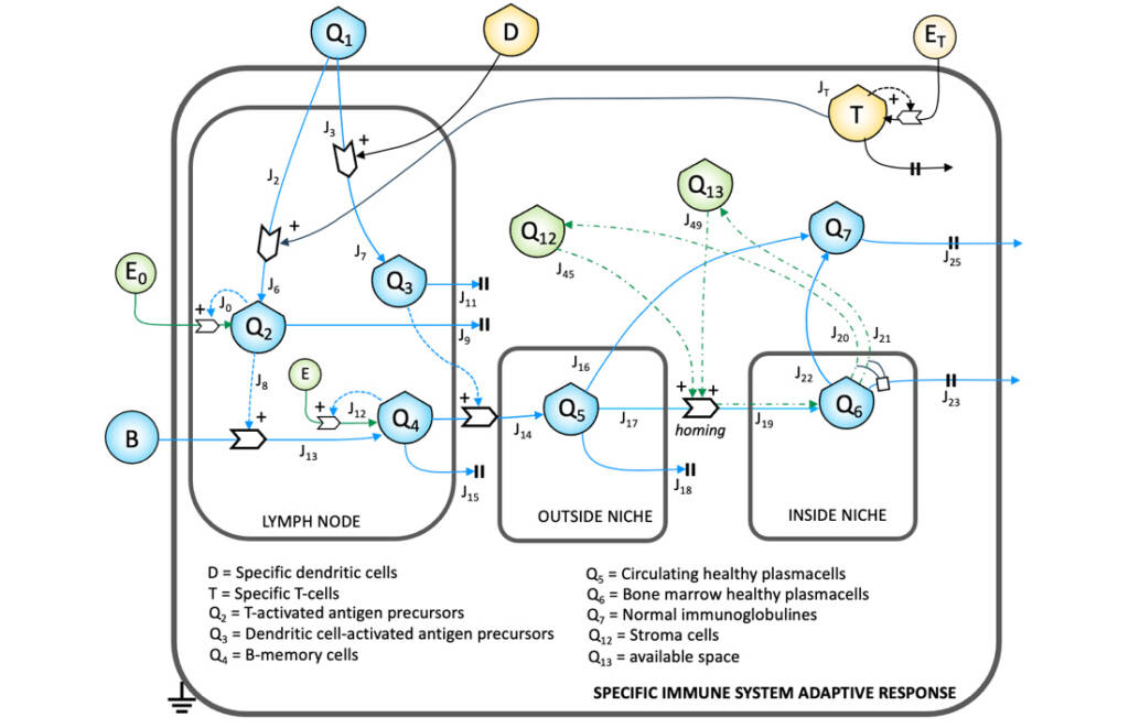
By setting up the corresponding differential equations, a computational simulator may be created, suitable to simulate the system dynamics and – most important – answer the “what if” questions. Figure 5 shows the state evolution of immune system representation of fig. 4, calculated by finite-difference methods starting from the analytical representation of the equations derived from the diagram (math not reported).
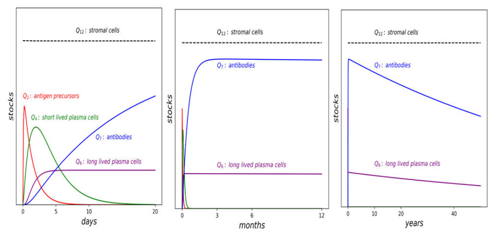
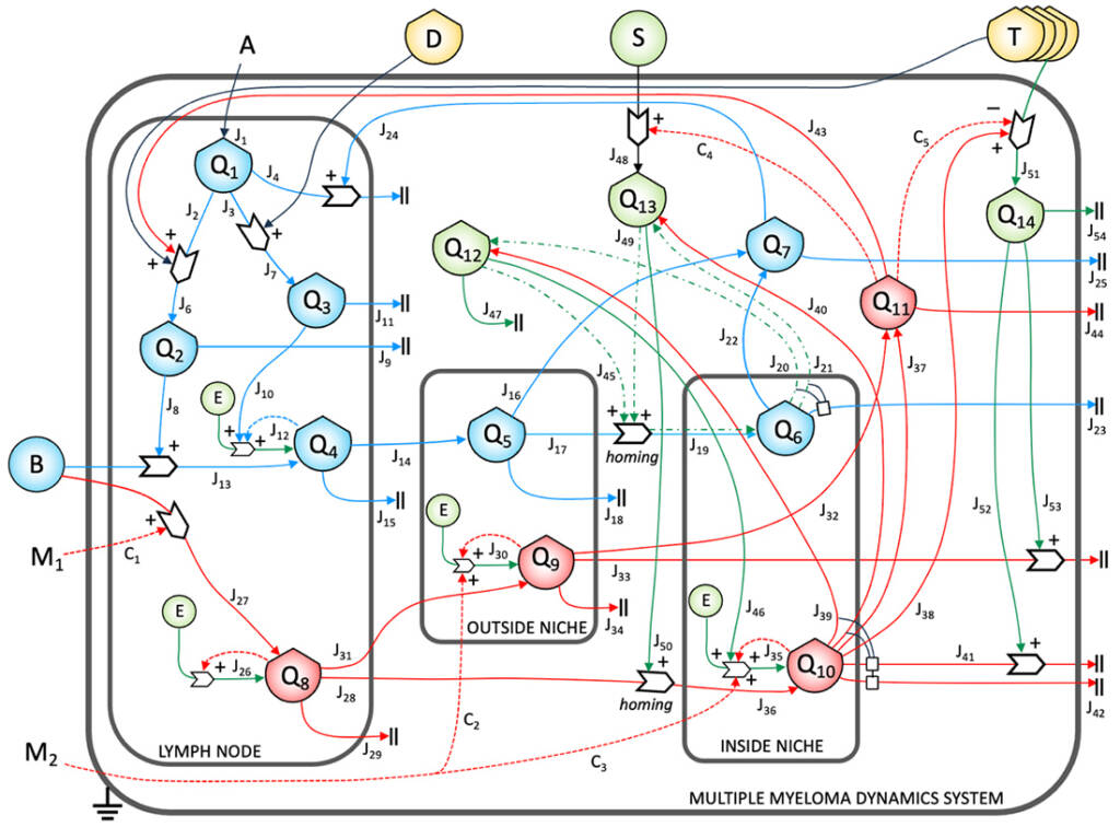
It must be remarked that this dynamics has been obtained without using free parameters, nor referring to any biochemical occurring in the system, but only starting from the knowledge of the mutual effect between the stocks, the knowledge of the biological parameters concerning the respective elements, and some reasonable assumption on the initial values for the stocks. In fact, the equation for a flow is not set to describe the change overtime of the flowing quantity, but rather its dependence on the state of the system, expressed by the set of values of the stocks, with no reference to the (supposedly non-linear) physical law that describes the flows in terms of physical quantities and usual phenomenological coefficients. This means that the structural model constituted by the equations may relate the states of the system (as expressed by the set of values for all the stocks) to points in the real spacetime, pointed out first by the trajectories of the system in its states space. This analytical approach is then substantiated by the mathematical expression(s) in the process where the flow(s) interact. Figure 6 shows as an example the state of the art of the ST diagram representation of Multiple Myeloma.
The proposed approach is at the same time profoundly abstract in nature and strongly connected to the experimental observation and activity. Nevertheless, more than clinical (big) data we aim at simulating the variety of dynamic behaviours of the disease, including the rearrangement following the action of external driving forces, such as drugs. Equations defined in the analytical model may be finally used to create a computational simulator, that correlates the states of the system at issue to an actual visualisation of its temporal dynamics.
The conceptual meaning of this procedure finds a parallel in the description of the chaotic dynamics of a system with a low number of degrees of freedom, but a high sensitivity to small variations in some parameter or variable. Even in that case, the dynamics cannot be studied starting from the physical laws that describe the actual (local) cause-effect relationships between the system elements, due to the unavailability of definite exact initial values. On the other hand, the description may use representations based on relatively simple recursive equations, that address the character of the system dynamics through its behaviour in terms of trajectories and attractors in the space of states. In our case, the conceptual role played by the recursivity of the chaotic equations is carried by the feedback loops, that become explicit by the very definition of the equations for the flows.
To do that with a prescribed degree of reliability, a set of initial data must be available, and a validation process must be defined. Calibration procedures use numerical values of flows (quantity processed per unit time) and stocks at a certain time, or possibly average data. Approximate plausible numbers are usually sufficient for starting, then, in an iterative procedure, the model is made run and calibration is refined. Steady-state conditions are also often used for calibration. In this case, missing values for flows are assumed as those necessary to make the inflows and outflows at a certain stock equal. A first run in of the model in steady state conditions should give straight or regularly oscillating lines. Figure 6 shows the workplan for application of ST to the quantitative study of a complex system.
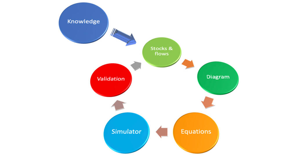
Models should be then validated in terms of accuracy to reality and usefulness, by techniques able to test their predictive capability, that must be accompanied by some validation procedure of the simulator setting up procedure. The study of how the disease system self-organizes, evolves and accesses different sets of configurations and patterns is one of the actual foci of the proposed approach. This means that the model itself will be set up by an iterative process: the scientific medical knowledge about a disease is used to draw a first version of the model in terms of all the stocks, flows and processes needed to represent the disease itself. This model is finally converted to a simulator, refined and integrated by testing its ability to simulate real data and the actual evolution of the disease under different initial conditions.
Being a stock-flow model based on extensive measurable variables, the procedure of validation must be seen therefore as a part of the setting up of the model itself. It is worth noticing that this procedure makes the complexity of the system an advantage for the model reliability validation. In fact, complex systems usually exhibit a great sensitivity to the change of external drivers, so the correctness of the simulator configuration will be tested by the capability of its output to reproduce real data, and its evolution in terms of variation of the system state.
